No items match. Try another category or clear the filters.
Launcher size
Welcome to the desktop
Use the launcher to browse categories, search for articles and applets, or narrow the list with Tags. The launcher starts pinned beside the desktop. Click its pin button to unpin it and give your windows more space; click Parks Computing in the top bar whenever you want to open it again.
Pick an article from the launcher and it opens as a floating window. Drag it by its title bar, resize it from any edge, snap it against the sides, or maximize it; open several and switch between them from the taskbar below. If you prefer windows to open maximized, choose that in Settings in the launcher.
Links inside an article open in their own windows, and so do the images; step through an article's images with the arrow keys, and pop one back down with Escape. The tags at the top of an article each open a window listing everything under that tag.
The whole arrangement lives in the page URL, so it can be bookmarked and shared, and Back undoes the last thing you did. Leave and come back, and the desktop resumes where you left off.
This view is built with PUDL, the Pleasantly Usable Design Language. Every article is still a page of its own; the ↗ button in a window's title bar takes you there.
Excel Employee Capacity Spreadsheet
· Updated
Excel Employee Capacity Spreadsheet
Once, when working for a professional-services organisation, I managed a team of business analysts and another team of software engineers. As professional-services employees, they were assigned to customer projects, sometimes more than one project at a time. Our organisation had KPIs for employee utilisation, so making sure employees were assigned to enough projects at the correct level was critical. At the same time, we also needed to reserve capacity for upcoming projects.
In order to be able to see utilisation and capacity at a glance, and also to be able to report on utilisation for monthly and quarterly business reviews, I developed an Excel spreadsheet that would display colourful graphs that could quickly reveal when employees were over- or under-utilised. It took a bit of Excel “kung fu” to accomplish this.
Since I've left that company, I no longer have that spreadsheet available, so I re-created it to share it here and explain the techniques that make it work. In this article, I'll walk the reader through the various worksheets, show how they fit together, and explain the formulas, table relationships, and formatting tricks that enable the graphical display.
In my old job, whenever a new project was confirmed, the project manager would contact the relevant line managers about the availability of needed resources. We would then look at how heavily loaded our staff were, and for how long they were committed to their current tasks. We needed a way to tell at a glance who was over-committed and who had enough slack to take on the assignment. Those were the primary needs that drove the development of the spreadsheet.
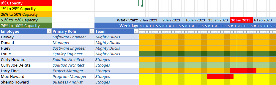
In the figure below, we can see that Louie, a Quality Engineer on the Mighty Ducks team, has at least 75% capacity. The rest of the Mighty Ducks team has from 26% to 50% capacity. The Stooges team has quite a bit less capacity. The red blocks beside Larry Fine and Moe Howard indicate dates when those employees will be out of office.
Employee capacity chart
Likewise, when it came time to evaluate where we stood vis-à-vis the utilisation metrics, the opposite at-a-glance view would be useful to tell us if we were tracking where we needed to or if we needed to find more work.
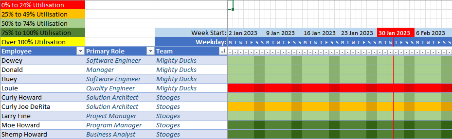
The figure below shows roughly the opposite view as the capacity chart. We now see a red bar next to Louie's name, indicating he is critically under-utilised. Curly Joe DeRita is a bit more engaged, and the rest of each team is at least at 50% utilisation.
Employee utilisation chart
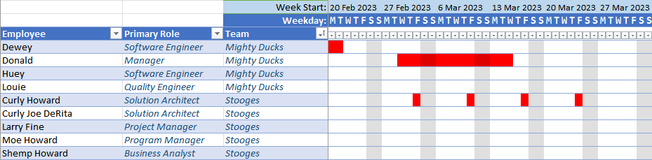
Finally, we needed to be able to account for scheduled time off. Although it was reflected in the capacity chart, it was also useful to view time off independently from project assignments.
First of all, any data of consequence is in a table. That's my primary rule for using Excel: If it's tabular data, put it into a table! Tables make editing, sorting, filtering, and correlating data vastly easier, and they also discourage some bad habits that can quickly make a mess of an otherwise tidy spreadsheet.
One big advantage of using tables is that you may use structured references to those tables when writing formulas. This lets you do table lookups, refer to entire columns, filter rows by column data in formulas, and so on. You'll see examples of this in the formulas below.
The main feature of this spreadsheet, though, is the graphical display of percentages. I use conditional formatting to achieve this by setting the text and background colours to the same colour, and varying the colour based on the value of the percentage.
Let's walk through all of the supporting tables, then things will make more sense when we get to the complicated formulas.
Set-Up Worksheets
The spreadsheet runs off of a number of tables, basically like a database. In fact, I'd like to develop a web app based on this spreadsheet at some point, but for now it's easy to prototype in Excel.
Teams
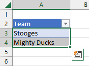
This table lists the names of the teams to which the employees belong. This could also be the names of the managers to which the employees report.
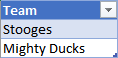
Teams table
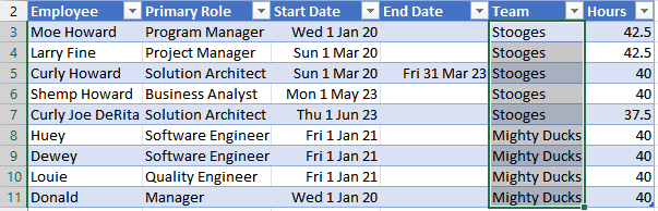
This is also used a data-validation list for the Team column in the Employees table. The way to set this up is to first select the column that should serve as a source list.
Select the source column
Next, assign a name to the list. If you add new rows to the table, the list will automatically expand to include those values.
Assign a name to the list
Next, select the column in the target table where you want data validation.
Select the target column
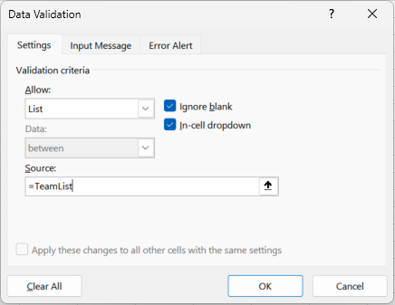
Finally, select the Data Validation command from the Data tab and enable list validation using the list name you just created.
Enable data validation using the named list
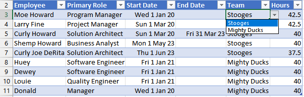
Now, when you edit a value in the column, a drop-down tab will appear with values from the validation list. You may also type values, but they will be validated against the list.
Values are selected from and compared against the list
This is used with several other columns throughout the spreadsheet. I'll call these out where relevant.
Roles
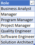
This table lists the various roles that employees may fill. Usually an employee will have a primary role, but they may also step into another role in a project, depending on the need.
Roles table
As with the Teams list, this is also a data-validation list for the Primary Role column in the Employees table.
Employees
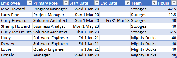
Now we're getting into the interesting bits. The Employees table contains all of the employees in the organisation whose utilisation should be tracked in our spreadsheet.
Employees table
As mentioned earlier, the Primary Role and Team columns are validated against the Roles and Teams tables.
The Primary Role is the role that the employee was hired to fill. It may be possible that an employee could fill a different role on a given project, however.
The Start Date is the date on which the employee commences work, and the End Date is the date when the employee will cease to work (if known). If there is no known end date, this column is blank.
The Hours column is the standard number of hours the employee works in a given week.
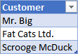
Customers
This table is just a list of customers that may have projects running. There could be additional columns in this table should you wish to track other details about your customers.
Customers table
Project Details
With all of the basic tables filled, we now move onto the project tables. These tables begin to combine the basic setup tables and show some of the special features of this spreadsheet.
Projects
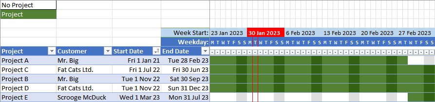
Now that we have our customer table, we can define the projects we have with those customers and their start and end dates. This table will demonstrate how the Gantt-chart representation of dates works.
Before we get to the chart portion of the table, we'll quickly cover the left-most data columns. Since we are tracking projects by customer, we need to define a unique project name, assign it to a customer, and set the start and end dates for the project. The Customer column is validated against the Customers table.
Project details table
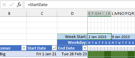
You'll notice the strip of dates above the top of the table that correspond to the beginning of each week. These dates drive the graphical chart. The left-most date cell refers to a cell on the “Home” worksheet that is labeled StartDate. The spreadsheet user sets this to the date from which the spreadsheet should report its timelines.
First week marker
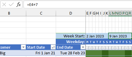
Every cell to the right is seven days greater to mark subsequent weeks.
Subsequent week marker
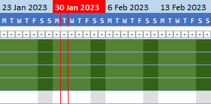
Next, you'll notice that the current week is highlighted in red, and the current day is bordered in red in all cells below that week.
Day and week highlighting
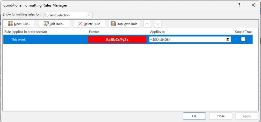
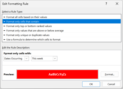
This is accomplished with conditional formatting. For the weekly cell, this is set up by selecting all the weekly cells across and creating a conditional-formatting rule.
Highlighting the current week
The rule is active for dates occurring in the current week, so the weekly cell that covers the current day will be highlighted with a red background and bold white text.
Custom format for highlighting the current week
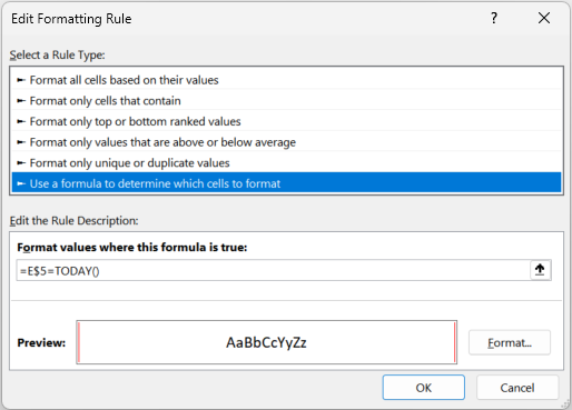
The red borders around the cells in the table for the current day are accomplished similarly, but with a formula. All of the cells on row 5 contain a formula that evaluates each cell to a day of the week in the weekly cell above it, but offset for the correct day of the week. These cells are then used to control formatting in the table below.
Select all of the table cells beneath the date cells and set a conditional-formatting rule that places a red border on either side of the cell, with the following formula:
=E$5=TODAY()
Cell E$5 is the first date cell, but since the column is relative and the row is absolute the effect is to test the date cell directly above each cell being formatted.
Adding red borders around the current day
Finally, there's a bit of a trick to displaying only the initial letter for each day of the week. If you select one of the standard date formats, the cell will only show “###” if the column width is too narrow to display the fully formatted date. If you make the column too narrow to even display a "#", you'll only see a blank cell.
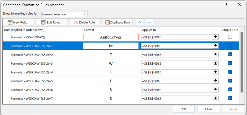
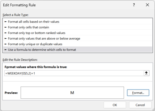
To work around this, we turn again to custom formatting. Select all of the day-of-week cells and create seven more conditional formats. Each is driven by a formula. For Mondays…
=WEEKDAY(E$5,2)=1
For Tuesdays…
=WEEKDAY(E$5,2)=2
...and so on.
Formatting days of the week
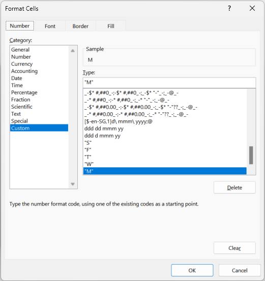
For each day, we set a custom format to display the exact letter desired for that day.
Using a formula to determine the day of the weekSetting a custom format for each day of the week
With these formats applied all the way across, with a small monospace font and a narrow column width, we're ready to work on the body of the Gantt chart.
Each cell in the table body underneath the day-of-week columns contains a formula like the one below. In each column, the E$5 cell reference will change to match the appropriate column, but everything else will remain the same.
The first thing this formula does is use the LET function to assign a name, thisDate, to the evaluation of cell E$5 (or the equivalent column).
=LET(thisDate, E$5,
The final parameter to the LET function is the calculation to execute. In this case, it uses the IF function to test three different conditions to make sure they are all TRUE. If they are, then it sets a value of 1 in the cell. If any of the values are not TRUE, it sets the cell to 0. The first test is to check if the Project column in the current row contains a value:
NOT(ISBLANK(ProjectTable[@[Project]:[Project]]))
The next test is whether the date in the End Date column in the current row is greater than or equal to the date of the column being evaluated:
ProjectTable[@[End Date]:[End Date]]>=thisDate
The final test is whether the date in the Start Date column in the current row is less than or equal to the date of the column being evaluated:
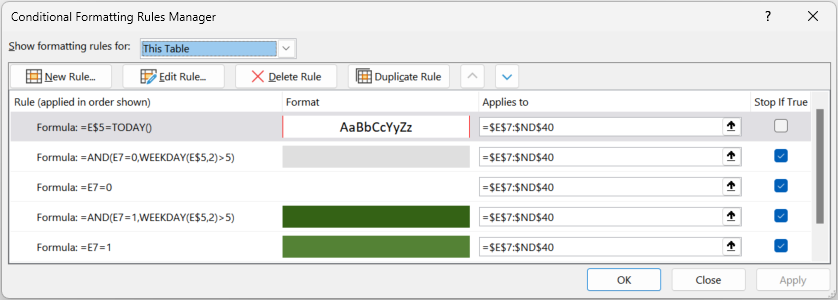
If all of the tests are true and the cell evaluates to 1, then we want to highlight the cell in dark green so that we can see that the project is active on that day. Again, we do this with conditional formatting. If you look again at the body of the table, you'll see vertical stripes that mark the weekends.
Project details table
To do this, we need two formats for when the cell contains a 0: when the date is a weekday, the background will be plain white, and when the date is a weekend it will be light grey. When the cell contains a 1, the backgrounds are dark green and darker green, respectively. We use formulas to determine the appropriate conditional format to use.
Formatting for weekdays and weekends
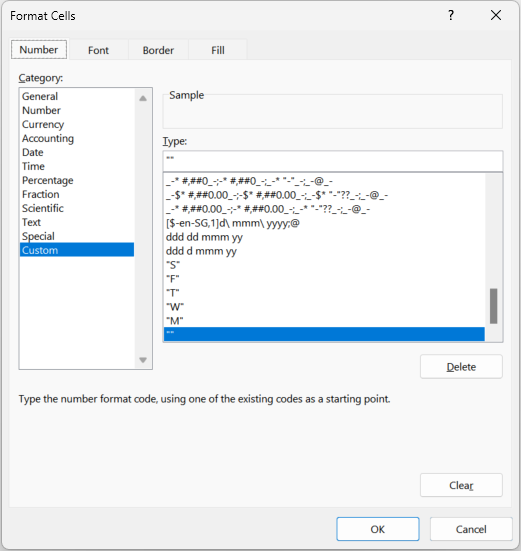
We also don't want to see “0” or “1” in each of the cells, so we also use a custom format to display a blank value.
Setting a blank foreground for Gantt-chart cells
Now we have all of the basic tools for creating a date-driven graphical table display. The rest of the worksheets build on the same basic formatting, but with percentage ranges rather than “1” or “0”.
Time Off Detail
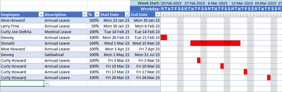
Each scheduled instance of time off is recorded in the Time Off Detail worksheet, by employee, listing the start and end date of each break. This is used in the Time-off Summary table and in the capacity table to show when an employee is unavailable for work. The Employee column is validated against the column of the same name in the Employees table.
Employee time-off detail
The rest of the worksheet is almost identical in structure to the Projects worksheet. The formula used in the body of the graphical display differs slightly from the Projects table, in that it reports a percentage value from the % column rather than “1”.
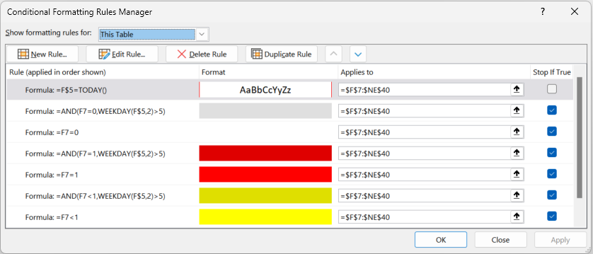
The conditional formatting for the graphical display also changes depending upon the percentage range. For values of 100%, the background color will be solid red. For values less than 100%, the background color will be yellow. As in the Projects table, the weekends will be highlighted in a darker color.
Varying background based on percentages
Each line in the table corresponds to one instance of time off, with a single start date and single end date. These will be consolidated in the Time Off Summary worksheet. For example, the four Fridays shown above as Annual Leave for Curly Howard will appear as follows in the summary sheet:
Employee time-off summary showing summarised time-off for Curly Howard
Assignments
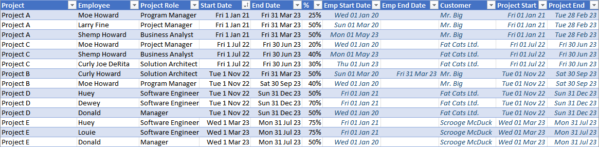
The Assignments table continues to build on the earlier tables we've discussed. In this table, employees defined in the Employees table are assigned to projects defined in the Projects table. Each assignment places an employee into a role on a project, with a start and end date and a percentage of commitment for the duration of the assignment. The Project, Employee, and Project Role columns are all validated against their respective definition tables.
You may have noticed that the seven right-most columns are all in dark-blue italic text. This is because these columns are calculated based on the other columns.
The Emp Start Date and Emp End Date columns are read from the Employees table using the name in the Employee column. This is done with the XLOOKUP function.
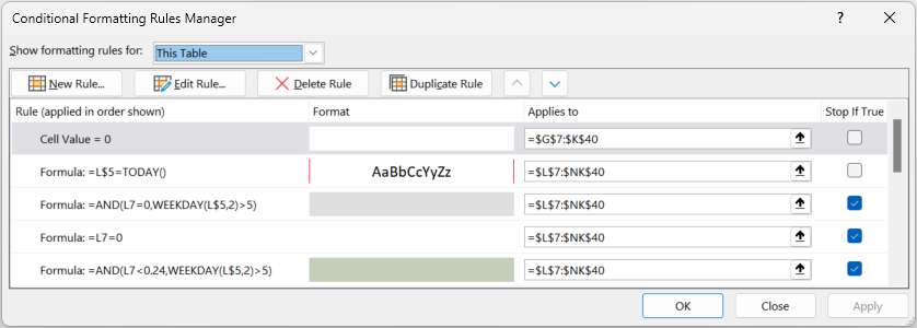
Since it is possible that an empty value could be returned from XLOOKUP and displayed as a 0, we use more conditional formatting so that these values are instead rendered as blanks.
Conditional formatting for values of zero
Then, for values of zero, just like in the body of the graphical display we use a custom format of "" so that there is no value shown in the cell.
Setting a blank foreground for Gantt-chart cells
Reporting Worksheets
Now that all of the project tables are set up, we can get to the real stars of the spreadsheet, which are the reporting worksheets. These tables use the same formatting techniques explained above, so we'll just look at the formulas used in the reporting.
Time Off Summary
When assigning staff to projects, it's helpful to see any scheduled time off for each staff member. This table summarises the individual entries in the Time Off Detail table to present a consolidated schedule of time off for all staff.
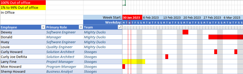
Employee time-off summary chart
The function in each cell of the table performs the following lookups for the employee in the current row to determine the value of the cell:
If employee's employment is terminated...
    Mark the employee as completely unavailable on this date.
Else...
    Find all employee entries in the Time-off Detail table.
    Of those entries, find the entries that begin on or before the date of the current cell.
    Of those entries, find the entries that end on or after the date of the current cell.
    Of those entries, sum the percentage of time off for the current date.
This logic translates to the following Excel formula placed in each cell of the graphical portion of the table. The variables thisDate, employee, endDate, and terminated are defined prior to the evaluation of the IF formula.
Any cell containing a percentage of 100% (or greater, if that happens) is shown as a red cell. Percentages from 1% to 99% are shown as yellow, and the rest are shown as blank.
Utilisation
The Utilisation table shows how much each employee is being utilised across various projects. This table summarises the Assignment table to present the current utilisation for each employee. In this spreadsheet, optimal utilisation is between 75% and 100%. This may vary in other organisations, of course.
Employee utilisation chart
The function in each cell of the table performs the following lookups for the employee in the current row to determine the value of the cell:
Find all employee entries in the Assignments table.
Of those entries, find the entries that begin on or before the date of the current cell.
Of those entries, find the entries that end on or after the date of the current cell.
Of those entries, sum the percentage of time assigned for the current date.
This logic translates to the following Excel formula placed in each cell of the graphical portion of the table.
The Capacity table reports how free each employee is to take on new tasks. This table summarises the Assignment table and the Time Off Detail to present the available capacity for each employee.
Employee capacity chart
The function in each cell of the table performs the following lookups for the employee in the current row to determine the value of the cell:
If employee's employment is terminated...
    Mark the employee as completely unavailable on this date.
Else...
    Sum this percentage...
        Find all employee entries in the Assignments table.
        Of those entries, find the entries that begin on or before the date of the current cell.
        Of those entries, find the entries that end on or after the date of the current cell.
        Of those entries, sum the percentage of time assigned for the current date.
    With this percentage...
        Find all employee entries in the Time-off Detail table.
        Of those entries, find the entries that begin on or before the date of the current cell.
        Of those entries, find the entries that end on or after the date of the current cell.
        Of those entries, sum the percentage of time off for the current date.
This logic translates to the following Excel formula placed in each cell of the graphical portion of the table.
 PUDL Theme Studio
 Barcode Scanner
 Barcode Tool
 Terminal
 Files
 Editor
 Diff Viewer
 Sight Reader
 Dice
 Sudoku
 Conway's Game of Life
 Barcode Flash Cards
 Asteroids
 Space Invaders